Premade estimator:

We used to .pop() function to split the label from the dataset. The label column name is called ‘Species’.

DNNEstimator(head, hidden_units, feature_columns, model_dir=None, optimizer=’Adagrad’, activation_fn=tf.nn.relu, dropout=None, config=None, warm_start_from=None, batch_norm=False)

BaselineEstimatorhead(model_dir=None, optimizer=’Ftrl’, config=None)

BoostedTreesEstimator( feature_columns, n_batches_per_layer, head, model_dir=None, weight_column=None, n_trees=100, max_depth=6, learning_rate=0.1, l1_regularization=0.0, l2_regularization=0.0, tree_complexity=0.0, min_node_weight=0.0, config=None, center_bias=False, pruning_mode=’none’, quantile_sketch_epsilon=0.01)

LinearEstimator( head, feature_columns, model_dir=None, optimizer=’Ftrl’, config=None, sparse_combiner=’sum’)

LinearRegessor( feature_columns, model_dir=None, label_dimension=1, weight_column=None, optimizer=’Ftrl’, config=None, warm_start_from=None, loss_reduction=losses_utils.ReductionV2.SUM_OVER_BATCH_SIZE, sparse_combiner=’sum’ )

Input functions are for importing data for training, testing, and predicting. Feature columns are for telling the model what feature you want to use.

classifier.train() trains the estimator model. It has two inputs- input_fn and steps. input_fn is a function we defined earlier in the code, which batches our data. We call that function so the classifier is trained on batches that the function creates. Steps specifies how long the model should train for.

DNNClassifier:

Test set accuracy: 0.800

Prediction is “Setosa” (78.5%), expected “Setosa”

Prediction is “Versicolor” (42.0%), expected “Versicolor”

Prediction is “Virginica” (61.0%), expected “Virginica”

LinearClassifier:

Test set accuracy: 0.933

Prediction is “Setosa” (87.5%), expected “Setosa”

Prediction is “Versicolor” (55.1%), expected “Versicolor”

Prediction is “Virginica” (65.2%), expected “Virginica”

DNNLinearCombinedClassifier:

Test set accuracy: 0.967

Prediction is “Setosa” (90.7%), expected “Setosa”

Prediction is “Versicolor” (64.2%), expected “Versicolor”

Prediction is “Virginica” (68.0%), expected “Virginica”

The DNNLinearCombinedClassifier worked the best. LinearClassifier was the second best, and DNNClassifier was the worst.

Build a Linear Model:

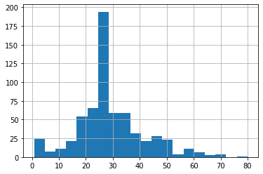
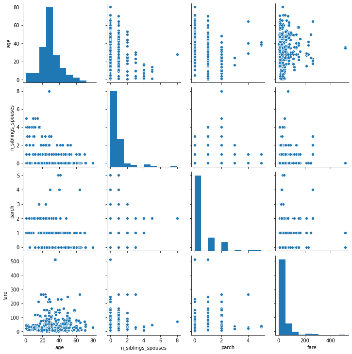
The data in the pairplot is more skewed right than it is in the regular histogram, but overall the distribution of age are pretty similar.

Categorical columns are the feature types of the variable, they have non-numerical inputs. Dense features have numeric inputs that are not used to classify a category.

The feature columns are ‘sex’, ‘n_siblings_spouses’, ‘parch’, ‘class’, ‘deck’, ‘embark_town’, ‘alone’, ‘age’, ‘fare’ The dense features of the list are ‘n_siblings_spouses’, ‘parch’ (number of parents/children on board), ‘age’, ‘fare’ The categorical features are ‘sex’, ‘class’, ‘deck’, ‘embark_town’, ‘alone’

The accuracy was 0.75757575 and the loss was 0.47347313. The model isn’t the best or most accurate. {‘accuracy’: 0.75757575, ‘accuracy_baseline’: 0.625, ‘auc’: 0.83330274, ‘auc_precision_recall’: 0.77572364, ‘average_loss’: 0.4817905, ‘label/mean’: 0.375, ‘loss’: 0.47347313, ‘precision’: 0.6666667, ‘prediction/mean’: 0.38785315, ‘recall’: 0.7070707, ‘global_step’: 200}

The purpose of adding a cross featured column to the model is to learn the differences between different feature combinations. Capturing the interaction between gender and age made the model worse. {‘accuracy’: 0.7462121, ‘accuracy_baseline’: 0.625, ‘auc’: 0.83489436, ‘auc_precision_recall’: 0.7468673, ‘average_loss’: 0.555922, ‘label/mean’: 0.375, ‘loss’: 0.5499551, ‘precision’: 0.7962963, ‘prediction/mean’: 0.23539768, ‘recall’: 0.43434343, ‘global_step’: 200}

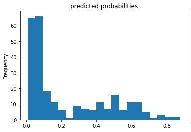
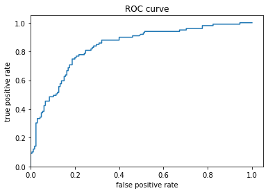
The plots below show the tradeoff between the true positive rate and the false positive rate